1. Introduction
This package aims to provide R users with a new way of accessing official Peruvian cartographic data on various topics that are managed by the country’s Spatial Data Infrastructure.
By offering a new approach to accessing this official data, both from technical-scientific entities and from regional and local governments, it facilitates the automation of processes, thereby optimizing the analysis and use of geospatial information across various fields.
However, this project is still under construction, for more information you can visit the GitHub official repository https://github.com/ambarja/geoidep.
If you want to support this project, you can support me with a coffee for my programming moments.
2. Package installation
install.packages("geoidep")Also, you can install the development version as follows:
install.packages('pak')
pak::pkg_install('ambarja/geoidep')3. Basic usage
providers <- get_data_sources()
providers
#> # A tibble: 83 × 7
#>    provider  category   layer layer_can_be_actived admin_en year  link_geoportal
#>    <chr>     <chr>      <chr> <lgl>                <chr>    <chr> <chr>
#>  1 INEI      General    depa… TRUE                 Nationa… 2019  https://ide.i…
#>  2 INEI      General    prov… TRUE                 Nationa… 2019  https://ide.i…
#>  3 INEI      General    dist… TRUE                 Nationa… 2019  https://ide.i…
#>  4 Midagri   Agricultu… agri… TRUE                 Ministr… 2024  https://siea.…
#>  5 Midagri   Agricultu… oil_… TRUE                 Ministr… 2016… https://siea.…
#>  6 Geobosque Forest     stoc… FALSE                Ministr… 2001… https://geobo…
#>  7 Geobosque Forest     stoc… TRUE                 Ministr… 2001… https://geobo…
#>  8 Geobosque Forest     stoc… TRUE                 Ministr… 2001… https://geobo…
#>  9 Geobosque Forest     stoc… TRUE                 Ministr… 2001… https://geobo…
#> 10 Geobosque Forest     warn… TRUE                 Ministr… last… https://geobo…
#> # ℹ 73 more rows
layers_available <- get_providers()
layers_available
#> # A tibble: 10 × 2
#>    provider         layer_count
#>    <fct>                  <int>
#>  1 Geobosque                  5
#>  2 INAIGEM                    5
#>  3 INEI                       7
#>  4 MapBiomas Alerta           1
#>  5 Midagri                    2
#>  6 MTC                       26
#>  7 Senamhi                    1
#>  8 Serfor                     1
#>  9 Sernanp                   31
#> 10 SIGRID                     4
4. Download Official Administrative Boundaries by INEI
# Region boundaries download
loreto_prov <- get_provinces(show_progress = FALSE) |>
  subset(nombdep == 'LORETO')
library(leaflet)
#>
#> Attaching package: 'leaflet'
#> The following object is masked _by_ '.GlobalEnv':
#>
#>     providers
library(sf)
#> Linking to GEOS 3.12.1, GDAL 3.8.4, PROJ 9.4.0; sf_use_s2() is TRUE
loreto_prov |>
  leaflet() |>
  addTiles() |>
  addPolygons()
# Defined Ubigeo
loreto_prov[["ubigeo"]] <- paste0(loreto_prov[["ccdd"]],loreto_prov[["ccpp"]])
# The first five rows
head(loreto_prov)
#> Simple feature collection with 6 features and 6 fields
#> Geometry type: MULTIPOLYGON
#> Dimension:     XY
#> Bounding box:  xmin: -76.89454 ymin: -8.715191 xmax: -69.94904 ymax: -0.63937
#> Geodetic CRS:  WGS 84
#>     ccdd ccpp                nombprov                     fuente nombdep
#> 138   16   01                  MAYNAS V Censo Nacional Economico  LORETO
#> 139   16   02           ALTO AMAZONAS V Censo Nacional Economico  LORETO
#> 140   16   03                  LORETO V Censo Nacional Economico  LORETO
#> 141   16   04 MARISCAL RAMON CASTILLA V Censo Nacional Economico  LORETO
#> 142   16   05                 REQUENA V Censo Nacional Economico  LORETO
#> 143   16   06                 UCAYALI V Censo Nacional Economico  LORETO
#>                               geom ubigeo
#> 138 MULTIPOLYGON (((-75.24086 -...   1601
#> 139 MULTIPOLYGON (((-76.30752 -...   1602
#> 140 MULTIPOLYGON (((-75.74592 -...   1603
#> 141 MULTIPOLYGON (((-72.08996 -...   1604
#> 142 MULTIPOLYGON (((-73.42087 -...   1605
#> 143 MULTIPOLYGON (((-74.82778 -...   1606
5. Working with Geobosque data
my_fun <- function(x){
  data <- get_forest_loss_data(
    layer = 'stock_bosque_perdida_provincia',
    ubigeo = loreto_prov[["ubigeo"]][x],
    show_progress = FALSE )
  return(data)
}
historico_list <- lapply(X = 1:nrow(loreto_prov),FUN = my_fun)
historico_df <- do.call(rbind.data.frame,historico_list)
# The first five rows
head(historico_df)
#>   anio perdida rango1 rango2 rango3  rango4  rango5 tipobosque ubigeo
#> 1 2001 4111.83      0   0.00 288.54 1387.08 2436.21          1   1601
#> 2 2002 2014.11      0   0.00 101.34  538.92 1373.85          1   1601
#> 3 2003 1448.01      0   0.00  60.66  386.91 1000.44          1   1601
#> 4 2004 3741.30      0   0.00 139.59 1344.42 2257.29          1   1601
#> 5 2005 3749.40      0   0.00 266.94 1213.38 2269.08          1   1601
#> 6 2006 1405.44      0  58.68  43.38  347.31  956.07          1   1601
6. Simple visualization with ggplot
library(ggplot2)
library(dplyr)
#>
#> Attaching package: 'dplyr'
#> The following objects are masked from 'package:stats':
#>
#> filter, lag
#> The following objects are masked from 'package:base':
#>
#> intersect, setdiff, setequal, union
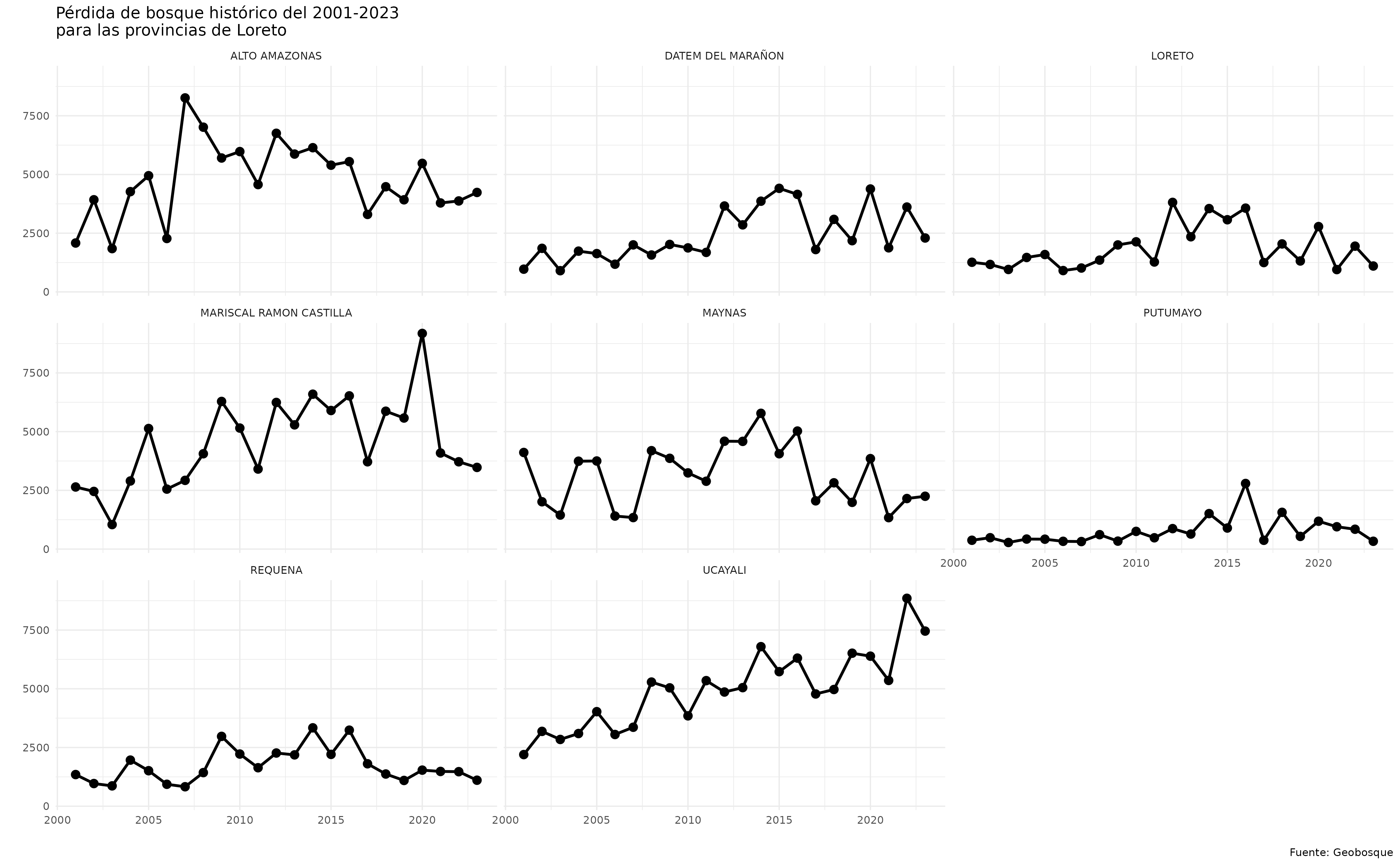
historico_df |>
inner_join(y = loreto_prov,by = "ubigeo") |>
ggplot(aes(x = anio,y = perdida)) +
geom_point(size = 1) +
geom_line() +
facet_wrap(nombprov~.,ncol = 3) +
theme_minimal(base_size = 5) +
labs(
title = "Pérdida de bosque histórico del 2001-2023 \npara las provincias de Loreto",
caption = "Fuente: Geobosque",
x = "",
y = "")